Deep Learning + Remote Sensing - Using NNs to turn imagery into meaningful features

Every now and again, the World Bank conducts something called a Living Standards Measurement Study (LSMS) survey in different countries, with the purpose being to learn about people, their incomes and expenses, how they’re doing economically and so on. These surveys provide very useful info to various stakeholders, but they’re expensive to conduct. What if we could estimate some of the parameters they measure from satellite imagery instead? That was the goal of some researchers at Stanford back in 2016, who came up with a way to do just that and wrote it up into this wonderful paper in Science. In this blog post, we’ll explore their approach, replicate the paper (using some more modern tools) and try a few experiments of our own.

Predicting Poverty: Where do you start?

Nighttime lights

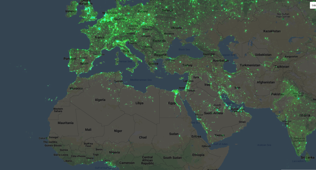
How would you use remote sensing to estimate economic activity for a given location? One popular method is to look at how much light is being emitted there at night - as my 3 regular readers may remember, there is a great nighttime lights dataset produced by NOAA that was featured in a data glimpse a while back. It turns out that the amount of light sent out does correlate with metrics such as assets and consumption, and this data has been used in the past to model things like economic activity (see another data glimpse post for more that). One problem with this approach: the low end of the scale gets tricky - nighttime lights don’t vary much below a certain level of expenditure.

Looking at daytime imagery, we see many things that might help tell us about the wealth in a place: type of roofing material on the houses, the number of roads, how built-up an area is…. But there’s a problem here too: these features are quite complicated, and training data is sparse. We could try to train a deep learning model to take in imagery and spit out income level, but the LSMS surveys typically only cover a few hundred locations - not a very large dataset, in other words.

Jean et al’s sneaky trick

The key insight in the paper is that we can train a CNN to predict nighttime lights (for which we have plentiful data) from satellite imagery, and in the process it will learn features that are important for predicting lights - and that these features will likely also be good for predicting our target variable as well! This multi-step transfer learning approach did very well, and is a technique that’s definitely worth keeping in mind when you’re facing a problem without much data.

But wait, you say. How is this better than just using nightlights? From the article: “How might a model partially trained on an imperfect proxy for economic well-being—in this case, the nightlights used in the second training step above—improve upon the direct use of this proxy as an estimator of well-being? Although nightlights display little variation at lower expenditure levels (Fig. 1, C to F), the survey data indicate that other features visible in daytime satellite imagery, such as roofing material and distance to urban areas, vary roughly linearly with expenditure (fig. S2) and thus better capture variation among poorer clusters. Because both nightlights and these features show variation at higher income levels, training on nightlights can help the CNN learn to extract features like these that more capably capture variation across the entire consumption distribution.” (Jean et al, 2016). So the model learns expenditure-dependent features that are useful even at the low end, overcoming the issue faced by approaches that use nightlights alone. Too clever!

Can we replicate it?

The authors of the paper shared their code publicly but… it’s a little hard to follow, and is scattered across multiple R and Python files. Luckily, someone has already done some of the hard work for us, and has shared a pytorch version in this GitHub repository. If you’d like to replicate the paper exactly, that’s a good place to start. I’ve gone a step further and consolidated everything into a single Google Colab notebook that borrows code from the above and builds on it. The rest of this post will explain the different sections of the notebook, and why I depart from the exact method used in the paper. Spoiler: we get a slightly better result with much fewer images downloaded.

Getting the data

The data comes from the Fourth Integrated Household Survey 2016-2017. We’ll focus on Malawi for this post. The notebook shows how to read in several of the CSV files downloaded from the website, and combine them into ‘clusters’ - see below. For each cluster location, we have a unique ID (HHID), a location (lat and lon), an urban/rural indicator, a weighting for statisticians, and the important variable: consumption (cons). This last one is the thing we’ll be trying to predict.

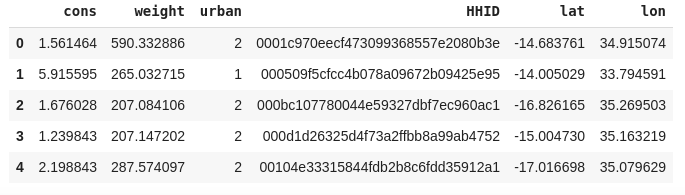
The relevant info from the survey data

One snag: the lat and lon columns are tricksy! They’ve been shifted to protect anonymity, so we’ll have to consider a 10km buffer around the given location and hope the true location is close enough that we get useful info.

Adding nighttime lights

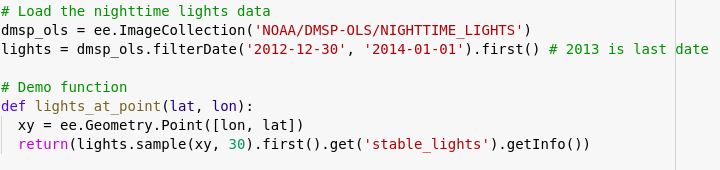
Getting the nightlights value for a given location

To get the nightlight data, we’ll use the python library to run Google Earth Engine queries. You’ll need a GEE account, and the notebook shows how to authenticate and get the required data. We can get the nightlights for each cluster location (getting the mean over an 8km buffer around the lat/lon points) and add this number as a column. To give us a target to aim at, we’ll compare any future models to a simple model based on these nightlight values only.

Downloading static maps images

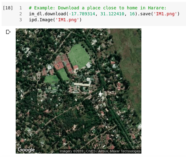
Getting imagery for a given location

The next step takes a while: we need to download images for the locations. BUT: we don’t just want one for each cluster location - instead, we want a selection from the surrounding area. Each of these will have it’s own nightlights value, so that we get a larger training set to build our model on. Later, we’ll extract features for each image in a cluster and combine them. Details are in the notebook. The code takes several hours to run, but at the end of it you’ll have thousands of images ready to use.

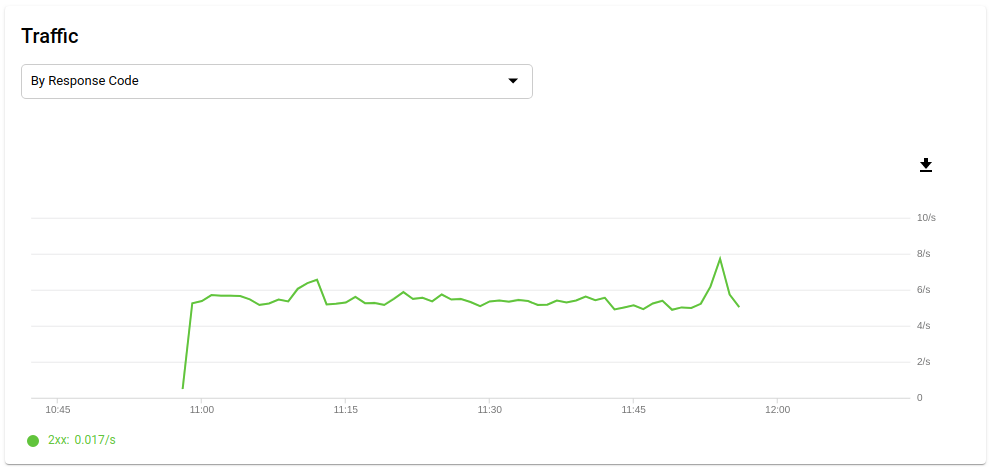
Tracking requests/sec on in my Google Cloud Console

You’ll notice that I only generate 20 locations around each cluster. The original paper uses 100. Reasons: 1) I’m impatient. 2) There is a rate limit of 25k images/day, and I didn’t want to wait (see #1), 3) The images are 400 x 400, but are then shrunk to train the model. I figured I could split the 400px image into 4 (or 9) smaller images that overlap slightly, and thus get more training data for free. This is suggested as a “TO TRY” in the notebook, but hint: it works. If you really wanted to get a better score, trying this or adding more imagery is an easy way to do so.

Training a model

I’ll be using fastai to simplify the model creation and training stages. before we can create a model, we need an appropriate databunch to hold the training data. An optional addition at this stage is to add image transforms to augment our training data - which I do with tfms = get_transforms(flip_vert=True, max_lighting=0.1, max_zoom=1.05, max_warp=0.) as suggested in the fastai satelite imagery example based on Planet labs. The notebook has the full code for creating the databunch:

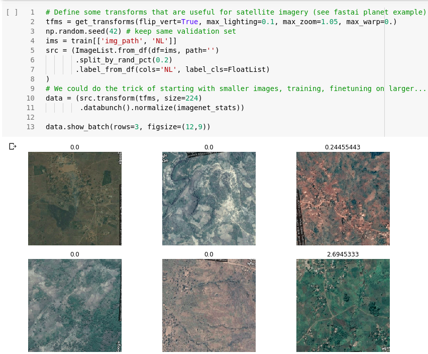
Data ready for modelling

Next, we choose a pre-trained model and re-train it with our data. Remember, the hope is that the model will learn features that are related to night lights and, by extension, consumption. I’ve had decent results with resnet models, but in the shared notebook I stick with models.vgg11_bn to more closely match the original paper. You could do much more on this model training step, but we pick a learning rate, train for a few epochs and move on. Another place to improve!

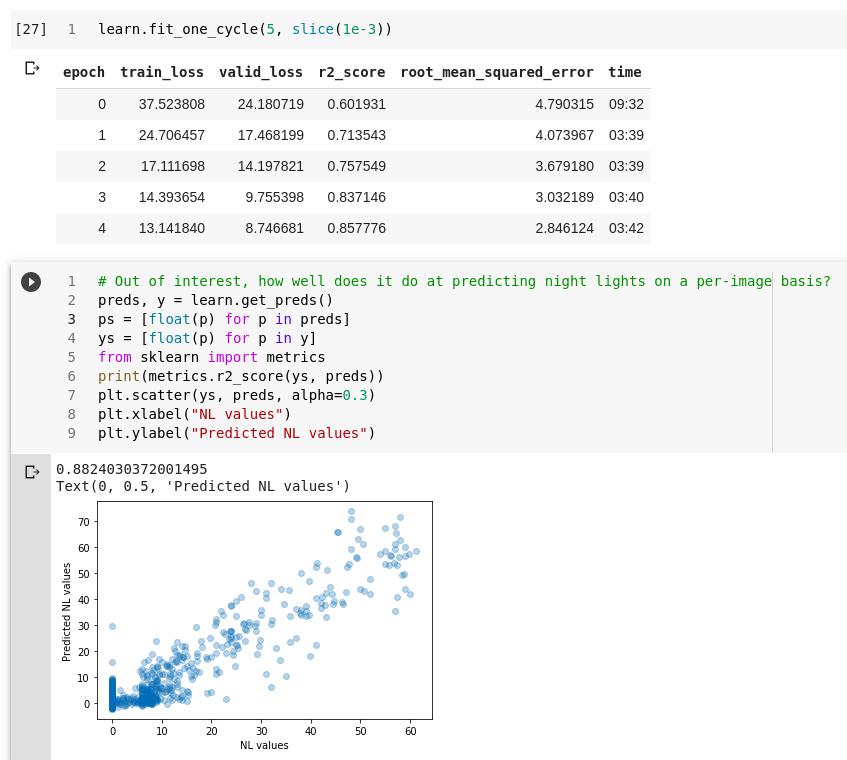
Training the model to predict nightlights

Using the model as a feature extractor

This is a really cool trick. We’ll hook into one of the final layers of the network, with 512 outputs. We’ll save these outputs as each image is run through the network, and they’ll be used in later modelling stages. To save the features, you could remove the last few layers and run the data through, or you can use a trick I learnt from this TDS article and keep the network intact.

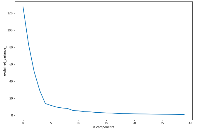
Cumulative explained variance of top PCA features

512 (or 4096, depending on the mode and which layer you pick) is a lot of features. So we use PCA to get 30 or so meaningful features from those 512 values. As you can see from the plot above, the top few components explain most of the variance in the data. These top 30 PCA components are the features we’ll use for the last step in the process: predicting consumption.

Putting it all together

For each image, we now have a set of 30 features that should be meaningful for predicting consumption. We group the images by cluster (aggregating their features). Now, for each cluster, we have the target variable (‘cons’), the nighttime lights (‘nl’) and 30 other potentially useful features. As we did right at the start, we’ll split the data into a test and a train set, train a model and then make predictions to see how well it does. Remember: our goal is to be better than a model that just uses nighttime lights. We’ll use the r^2 score when predicting log(y), as in the paper. The results:

• Score using just nightlights (baseline): 0.33
• Score with features extracted from imagery: 0.41

Using just the features derived from the imagery, we got a significant score increase. We’ve successfully used deep learning to squeeze some useful information out of satellite imagery, and in the process found a way to get better predictions of survey outcomes such as consumption. The paper got a score of 0.42 for Malawi using 100 images to our 20, so I’d call this a success.

Improvements

There are quite a few ways you can improve the score. Some are left as exercises for the reader :) here are a few that I’ve tried:
1) Tweaking the model used in the final step: 0.44 (better than the paper)
2) Using sub-sampling to boost size of training dataset + using a random forest model: 0.51 (!)
3) Using a model trained for classification on binned NL values (as in paper) as opposed to training it on a regression task: score got worse
4) Cropping the downloaded images into 4 to get more training data for the model (no other changes): 0.44 up from 0.41 without this step. >0.5 aggregating features of 3 different subsets of images for each cluster
5) Using a resnet-50 model: 0.4 (no obvious change this time - score likely depends less on model architecture and more on how well it is trained)

Other potential improvements:
- Download more imagery
- Train the model used as a feature extractor better (I did very little experimentation or fine-tuning)
- Further explore the sub-sampling approach, and perhaps make multiple predictions on different sub-samples for each cluster in the test set, and combine the predictions.

Please let me know if any of these work well for you. I’m less interested in spending more time on this - see the next section.

Where next

I’m happy with these results, but don’t like a few aspects:

• Using static maps from Google means we don’t know the date the imagery was acquired, and makes it hard to extend our predictions over a larger area without downloading a LOT of imagery (meaning you’d have to pay for the service or wait weeks)
• Using RGB images and an imagenet model means we’re starting from a place where the features are not optimal for the task - hence the need for the intermediate nighttime lights training step. It would be nice to have some sort of model that can interpret satellite imagery well already and go straight to the results.
• Downloading from Google Static Maps is a major bottleneck. I used only 20 images / cluster for this blog - to do 100 per cluster and for multiple countries would take weeks, and to extend predictions over Africa months. There is also patchy availability in some areas.

So, I’ve been experimenting with using Sentinel 2 imagery, which is freely available for download over large areas and comes with 13 bands over a wide spectrum of wavelengths. The resolution is lower, but the imagery still has lots of useful info. There are also large, labeled datasets like the EuroSAT database that have allowed people to pretrain models and achieve state of the art results for tasks like land cover classification. I’ve taken advantage of this by using a model pre-trained on this imagery for land cover classification tasks (using all 13 bands) and re-training it for use in the consumption prediction task we’ve just been looking at. I’ve been able to basically match the results we got above using only a single Sentinel 2 image for each cluster.

Using Sentinel imagery solves both my concerns - we can get imagery for an entire country, and make predictions for large areas, at different dates, without needing to rely on Google’s Static Maps API. More on this project in a future post…

Conclusion

As always, I’m happy to answer questions and explain things better! Please let me know if you’d like the generated features (to save having to run the whole modelling process), more information on my process or tips on taking this further. Happy hacking :)