Zindi UberCT Part 2: Stepping Up
In part 1, we looked at the SANRAL challenge on Zindi and got a simple first submission up on the leaderboard. In this tutorial I’ll show some extra features you can add on the road segments, bring in an external weather dataset, create a more complex model and give some hints on other things to try. Part 3 will hopefully add Uber movement data (waiting on the Oct 29 launch) and run through some GIS trickery to push this even further, but even without that you should be able to get a great score based on the first two tutorials.
You can follow along in the accompanying notebook, available here. Let’s dive in.
Reading a shapefile with GeoPandas
Reading the data from the road_segments shapefile
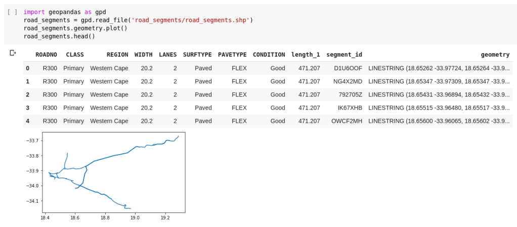
If you unzip the road_segments.zip file downloaded from Zindi (!unzip road_segments.zip), you’ll find a group of files with all sorts of weird extensions: .shp, .shx, .dbf, .cpg…. What is all this? This is a standard format for geospatial vector data known as a shapefile. The .shp file is the key, while the others add important extra info such as attributes and shape properties. Fortunately, we don’t have to deal with these different files ourselves - the geopandas library makes it fairly simple (see above). Once we have the data in a dataframe, all we need to do is merge on segment_id (train = pd.merge(train, road_segments, on='segment_id', how='left') to get some juicy extra info in our training set. These new features include the number of lanes, the surface type, the segment length and condition… all useful inputs to our model.
Finding weather data
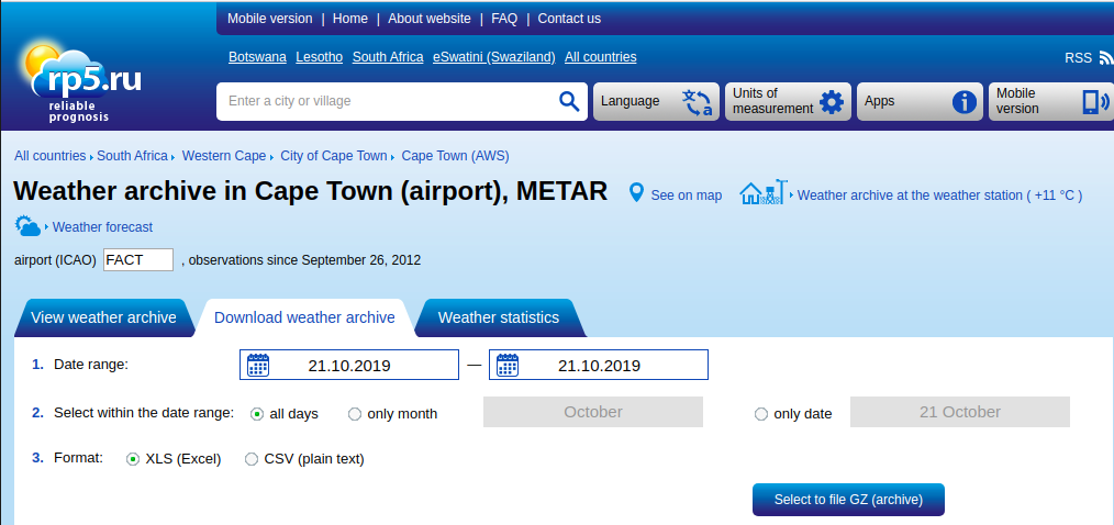
Zindi included a sentence on the data page: “You may use weather in your model. Please suggest weather datasets…”. I googled around and found rp5.ru - an excellent site that lets you download some historical weather data for locations around the globe. You’re welcome to check out the site, enter a date range, download, rename, etc. Or you can use my csv file, available here on github.
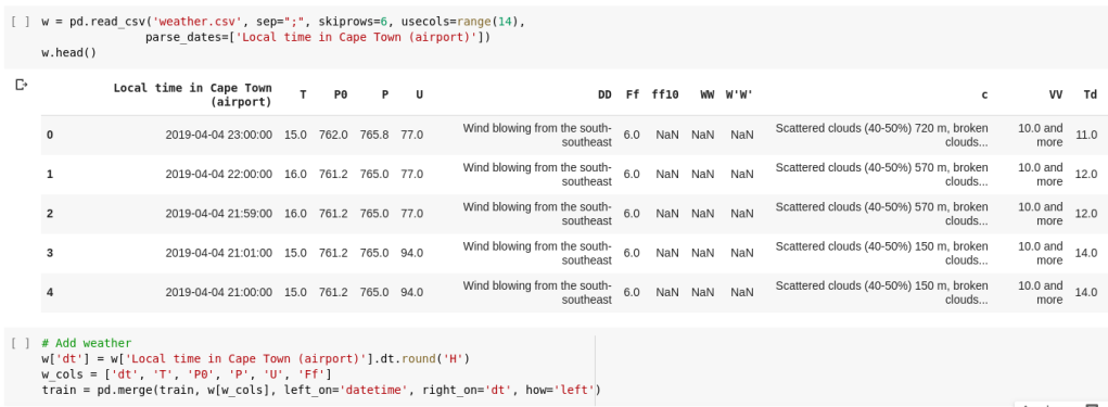
We can read the data from the CSV file and then link it to our training data with another simple merge command. The details are in the notebook. You can read about what the columns mean on the rp5.ru site. I the example I only use the numeric columns, but you could add extra features like wind direction, clouds_present etc based on the text components of this dataset.
Deep learning for tabular data
I’ve recently been playing around a lot with the incredible fastai library. The course (fast.ai) will get you going quickly, and I highly recommend running through some of the examples there. In one of the lessons, Jeremy shows the use of a neural network on tabular data. This was traditionally fairly hard, and you had to deal with embeddings, normalization, overfitting….. Recently however, I’m seeing more and more use of these models for tabular data, thanks in no small part to fastai’s implementation that handles a lot of the complexity for you.
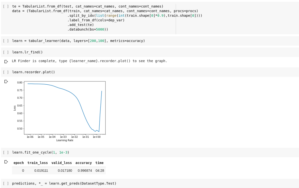
Using fastai’s tabular learner.
I was going to go in-depth here with a tutorial, but honestly you’d be better off going to the source and seeing a lesson from Jeremy Howard (founding researcher at fast.ai) who takes you through dealing with tabular data as part of the aforementioned course. The relevant lesson is lesson 4, but if you have a few hours I’d suggest starting from the beginning.
How far have we come, and where do we go next?
I haven’t talked much about model scores or performance in this post. Is it worth adding all this extra data? And do these fancy neural networks do anything useful? Yes and yes - by making the improvements described above we take our score from 0.036 to 0.096, placing us just behind the top few entries.
But we have a secret weapon: the additional data! This score is achieved without making use of the vehicle counts per zone, the incident records or the vehicle data from SANRAL, and we haven’t even looked at Uber Movement yet.
I’m going to wait on writing the next part of this series. So, dear reader (or readers, if this gets traction!), the baton lies with you. Add that extra data, get creative with your features, play with different models and let’s see how good we can get.